
sym2code knowledge base
Sym2Code Example
Check the control design via simulation before to deploy the final code.
Control Law Design
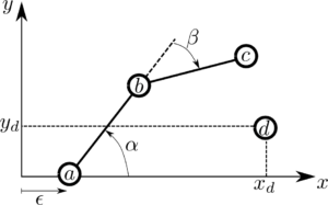
Let us consider the system depicted in picture.
The position of the three points of interest can be easily found as:
p_a = \begin{pmatrix} \epsilon \\ 0\end{pmatrix}
p_b = p_a + R_\alpha \begin{pmatrix} l_1 \\ 0\end{pmatrix}, \qquad R_\alpha = \begin{pmatrix} \cos \alpha & -\sin \alpha \\ \sin \alpha & \cos \alpha \end{pmatrix}
p_c = p_b + R_\alpha R_\beta \begin{pmatrix} l_2 \\ 0\end{pmatrix}, \qquad R_\beta = \begin{pmatrix} \cos \beta & -\sin \beta \\ \sin \beta & \cos \beta \end{pmatrix}
Considering the joint variables:
q = \begin{pmatrix} \epsilon, & \alpha, & \beta \end{pmatrix}^\top
we can formulate the control problem of finding the control law to reduce asymptotically the error: \tilde{p} = p_d – p_c(q) between a fixed position p_d \in \mathbb{R}^2 such that \dot{p}_d = 0 and the result of the direct kinematics represented by the function p_c(q): \mathbb{R}^3 \rightarrow \mathbb{R}^2.
Let us consider a Lyapunov function:
V(\tilde{p}) = \frac{1}{2} \tilde{p}^\top \tilde{p} \succ 0 \quad \forall \quad \tilde{p} \neq 0
computing the time derivative we obtain:
\dot{V}(\tilde{p}) = \tilde{p}^\top (-J(q)\dot{q}), \qquad J(q) =\frac{\partial p_c(q)}{\partial q}
where J(q) is the analytical Jacobian.
As the choice of the control action should enforce negative definiteness for the Lyapunov function time derivative, a possible choice can be immediately identified by:
\dot{q} = K J^\top(q) \left( p_d – p_c(q) \right)
It is well known that kinematics singularities might affect the control results as the matrix J(q) K J^\top(q) is responsible of the quadratic form:
\dot{V}(\tilde{p}) = -\tilde{p}^\top J(q) K J^\top(q) \tilde{p} \prec 0
A good indicator of the singularity proximity is given by the manipulability computed as:
\mu =det(J(q)J^\top(q))
Let us now convert our math results into runnable code with Sym2Code
Code Generation
% Joint variables
q = SymVectorCol('q',{'epsilon','alpha','beta'}, 'Joint State');

% Arms length
L = SymVectorCol('l',1:2, 'Link Length');

% Rotation matrices
R_alpha = [cos(q(2)), -sin(q(2)); sin(q(2)), cos(q(2))];
R_beta = [cos(q(3)), -sin(q(3)); sin(q(3)), cos(q(3))];

% Direct kinematics of the points of interest
p_a = Sym('p_a',[q(1);0],'Position A');
p_b = Sym('p_b',p_a + R_alpha*[L(1);0],'Position B');
p_c = Sym('p_c',simplify(p_b + R_alpha*R_beta*[L(2);0]),'Position C');

Sym2Code({p_a, p_b, p_c}, 'PRRKine', {q, L});

% Lyapunov control law
p_d = SymVectorCol('p_d',{'x','y'}, 'Desired Position');
K = SymVectorCol('K',{'x','alpha', 'beta'}, 'Gain');
J = Sym('J', simplify(jacobian(p_c,q)), 'Analytic Jacobian');
q_dot_c = Sym('u', simplify(diag(K)*J'*(p_d-p_c)), 'Kinematic Control');

Sym2Code({q_dot_c, J}, 'PRRCtrl', {q, L, p_d, K});
Resulting Code
PRRKine.m
function [p_a,p_b,p_c, bError] = PRRKine(q,l)
%-----------------------------------------------------------------------------
% This code has been automatically generated using Sym2Code Toolbox
% Sym2Code M Target
%-----------------------------------------------------------------------------
% WARNING: Modifying the following code is not recommended.
%-----------------------------------------------------------------------------
% For more information:
% - visit our webpage www.cybertronics.cloud
% - write an email to sym2code@cybertronics.cloud
%-----------------------------------------------------------------------------
% Inputs:
% q is a 3x1: Joint State */
% l is a 2x1: Link Length */
% Output:
% p_a is a 2x1: Position A */
% p_b is a 2x1: Position B */
% p_c is a 2x1: Position C */
%-----------------------------------------------------------------------------

% The module is named PRRKine and has 2 inputs and 3 outputs

p_a = zeros(2,1); % Output n. 1 is: Position A
p_b = zeros(2,1); % Output n. 2 is: Position B
p_c = zeros(2,1); % Output n. 3 is: Position C
bError = true;

XTmp = zeros(1,12); % Optimal Transition Variables

% Check input data

% Input n. 1 is: Joint State
if(isempty(q)), return; end
if(size(q,1)~=3), return; end
if(size(q,2)~=1), return; end
if(~isempty(q(isnan(q)==1))), return; end

% Input n. 2 is: Link Length
if(isempty(l)), return; end
if(size(l,1)~=2), return; end
if(size(l,2)~=1), return; end
if(~isempty(l(isnan(l)==1))), return; end

% Perform main calculation

% Computing cos(q_alpha) as
XTmp(1) = cos(q(2,1));
% Computing l_1*cos(q_alpha) as
XTmp(2) = (XTmp(1)*l(1,1));
% Computing q_epsilon + l_1*cos(q_alpha) as
XTmp(3) = (XTmp(2)+q(1,1));
% Computing sin(q_alpha) as
XTmp(4) = sin(q(2,1));
% Computing l_1*sin(q_alpha) as
XTmp(5) = (XTmp(4)*l(1,1));
% Computing q_alpha + q_beta as
XTmp(6) = (q(2,1)+q(3,1));
% Computing cos(q_alpha + q_beta) as
XTmp(7) = cos(XTmp(6));
% Computing l_2*cos(q_alpha + q_beta) as
XTmp(8) = (XTmp(7)*l(2,1));
% Computing q_epsilon + l_2*cos(q_alpha + q_beta) + l_1*cos(q_alpha) as
XTmp(9) = (XTmp(3)+XTmp(8));
% Computing sin(q_alpha + q_beta) as
XTmp(10) = sin(XTmp(6));
% Computing l_2*sin(q_alpha + q_beta) as
XTmp(11) = (XTmp(10)*l(2,1));
% Computing l_2*sin(q_alpha + q_beta) + l_1*sin(q_alpha) as
XTmp(12) = (XTmp(5)+XTmp(11));

% Generating optimal output for p_a which is p_a with comment: Position A
% as q_epsilon
p_a(1,1) = q(1,1);
% as 0
p_a(2,1) = 0.000000e+00;

% Generating optimal output for p_b which is p_b with comment: Position B
% as q_epsilon + l_1*cos(q_alpha)
p_b(1,1) = XTmp(3);
% as l_1*sin(q_alpha)
p_b(2,1) = XTmp(5);

% Generating optimal output for p_c which is p_c with comment: Position C
% as q_epsilon + l_2*cos(q_alpha + q_beta) + l_1*cos(q_alpha)
p_c(1,1) = XTmp(9);
% as l_2*sin(q_alpha + q_beta) + l_1*sin(q_alpha)
p_c(2,1) = XTmp(12);

% Return a valid state
bError = false;
end
PRRCtrl.m
function [u,J, bError] = PRRCtrl(q,l,p_d,K)
%-----------------------------------------------------------------------------
% This code has been automatically generated using Sym2Code Toolbox
% Sym2Code M Target
%-----------------------------------------------------------------------------
% WARNING: Modifying the following code is not recommended.
%-----------------------------------------------------------------------------
% For more information:
% - visit our webpage www.cybertronics.cloud
% - write an email to sym2code@cybertronics.cloud
%-----------------------------------------------------------------------------
% Inputs:
% q is a 3x1: Joint State */
% l is a 2x1: Link Length */
% p_d is a 2x1: Desired Position */
% K is a 3x1: Gain */
% Output:
% u is a 3x1: Kinematic Control */
% J is a 2x3: Analytic Jacobian */
%-----------------------------------------------------------------------------

% The module is named PRRCtrl and has 4 inputs and 2 outputs

u = zeros(3,1); % Output n. 1 is: Kinematic Control
J = zeros(2,3); % Output n. 2 is: Analytic Jacobian
bError = true;

XTmp = zeros(1,29); % Optimal Transition Variables

% Check input data

% Input n. 1 is: Joint State
if(isempty(q)), return; end
if(size(q,1)~=3), return; end
if(size(q,2)~=1), return; end
if(~isempty(q(isnan(q)==1))), return; end

% Input n. 2 is: Link Length
if(isempty(l)), return; end
if(size(l,1)~=2), return; end
if(size(l,2)~=1), return; end
if(~isempty(l(isnan(l)==1))), return; end

% Input n. 3 is: Desired Position
if(isempty(p_d)), return; end
if(size(p_d,1)~=2), return; end
if(size(p_d,2)~=1), return; end
if(~isempty(p_d(isnan(p_d)==1))), return; end

% Input n. 4 is: Gain
if(isempty(K)), return; end
if(size(K,1)~=3), return; end
if(size(K,2)~=1), return; end
if(~isempty(K(isnan(K)==1))), return; end

% Perform main calculation

% Computing q_alpha + q_beta as
XTmp(1) = (q(2,1)+q(3,1));
% Computing cos(q_alpha + q_beta) as
XTmp(2) = cos(XTmp(1));
% Computing l_2*cos(q_alpha + q_beta) as
XTmp(3) = (XTmp(2)*l(2,1));
% Computing cos(q_alpha) as
XTmp(4) = cos(q(2,1));
% Computing l_1*cos(q_alpha) as
XTmp(5) = (XTmp(4)*l(1,1));
% Computing -p_d_x as
XTmp(6) = (-p_d(1,1));
% Computing q_epsilon - p_d_x + l_2*cos(q_alpha + q_beta) + l_1*cos(q_alpha) as
XTmp(7) = (((XTmp(3)+XTmp(5))+XTmp(6))+q(1,1));
% Computing -K_x*(q_epsilon - p_d_x + l_2*cos(q_alpha + q_beta) + l_1*cos(q_alpha)) as
XTmp(8) = ((-K(1,1))*XTmp(7));
% Computing sin(q_alpha + q_beta) as
XTmp(9) = sin(XTmp(1));
% Computing l_2*sin(q_alpha + q_beta) as
XTmp(10) = (XTmp(9)*l(2,1));
% Computing sin(q_alpha) as
XTmp(11) = sin(q(2,1));
% Computing l_1*sin(q_alpha) as
XTmp(12) = (XTmp(11)*l(1,1));
% Computing l_2*sin(q_alpha + q_beta) + l_1*sin(q_alpha) as
XTmp(13) = (XTmp(10)+XTmp(12));
% Computing K_alpha*(l_2*sin(q_alpha + q_beta) + l_1*sin(q_alpha))*(q_epsilon - p_d_x + l_2*cos(q_alpha + q_beta) + l_1*cos(q_alpha)) as
XTmp(14) = ((K(2,1)*XTmp(7))*XTmp(13));
% Computing l_2*cos(q_alpha + q_beta) + l_1*cos(q_alpha) as
XTmp(15) = (XTmp(3)+XTmp(5));
% Computing -p_d_y as
XTmp(16) = (-p_d(2,1));
% Computing l_2*sin(q_alpha + q_beta) - p_d_y + l_1*sin(q_alpha) as
XTmp(17) = (XTmp(13)+XTmp(16));
% Computing -K_alpha*(l_2*cos(q_alpha + q_beta) + l_1*cos(q_alpha))*(l_2*sin(q_alpha + q_beta) - p_d_y + l_1*sin(q_alpha)) as
XTmp(18) = (((-K(2,1))*XTmp(15))*XTmp(17));
% Computing K_alpha*(l_2*sin(q_alpha + q_beta) + l_1*sin(q_alpha))*(q_epsilon - p_d_x + l_2*cos(q_alpha + q_beta) + l_1*cos(q_alpha)) - K_alpha*(l_2*cos(q_alpha + q_beta) + l_1*cos(q_alpha))*(l_2*sin(q_alpha + q_beta) - p_d_y + l_1*sin(q_alpha)) as
XTmp(19) = (XTmp(18)+((K(2,1)*XTmp(13))*((XTmp(6)+XTmp(15))+q(1,1))));
% Computing p_d_y*cos(q_alpha + q_beta) as
XTmp(20) = (XTmp(2)*p_d(2,1));
% Computing q_epsilon*sin(q_alpha + q_beta) as
XTmp(21) = (XTmp(9)*q(1,1));
% Computing sin(q_beta) as
XTmp(22) = sin(q(3,1));
% Computing l_1*sin(q_beta) as
XTmp(23) = (XTmp(22)*l(1,1));
% Computing -p_d_x*sin(q_alpha + q_beta) as
XTmp(24) = (XTmp(6)*XTmp(9));
% Computing p_d_y*cos(q_alpha + q_beta) - p_d_x*sin(q_alpha + q_beta) + q_epsilon*sin(q_alpha + q_beta) + l_1*sin(q_beta) as
XTmp(25) = (((XTmp(20)+XTmp(21))+XTmp(23))+XTmp(24));
% Computing K_beta*l_2*(p_d_y*cos(q_alpha + q_beta) - p_d_x*sin(q_alpha + q_beta) + q_epsilon*sin(q_alpha + q_beta) + l_1*sin(q_beta)) as
XTmp(26) = ((K(3,1)*XTmp(25))*l(2,1));
% Computing -l_2*sin(q_alpha + q_beta) as
XTmp(27) = (-XTmp(10));
% Computing -l_1*sin(q_alpha) as
XTmp(28) = (-XTmp(12));
% Computing - l_2*sin(q_alpha + q_beta) - l_1*sin(q_alpha) as
XTmp(29) = (XTmp(27)+XTmp(28));

% Generating optimal output for u which is u with comment: Kinematic Control
% as -K_x*(q_epsilon - p_d_x + l_2*cos(q_alpha + q_beta) + l_1*cos(q_alpha))
u(1,1) = XTmp(8);
% as K_alpha*(l_2*sin(q_alpha + q_beta) + l_1*sin(q_alpha))*(q_epsilon - p_d_x + l_2*cos(q_alpha + q_beta) + l_1*cos(q_alpha)) - K_alpha*(l_2*cos(q_alpha + q_beta) + l_1*cos(q_alpha))*(l_2*sin(q_alpha + q_beta) - p_d_y + l_1*sin(q_alpha))
u(2,1) = XTmp(19);
% as K_beta*l_2*(p_d_y*cos(q_alpha + q_beta) - p_d_x*sin(q_alpha + q_beta) + q_epsilon*sin(q_alpha + q_beta) + l_1*sin(q_beta))
u(3,1) = XTmp(26);

% Generating optimal output for J which is J with comment: Analytic Jacobian
% as 1
J(1,1) = 1.000000e+00;
% as - l_2*sin(q_alpha + q_beta) - l_1*sin(q_alpha)
J(1,2) = XTmp(29);
% as -l_2*sin(q_alpha + q_beta)
J(1,3) = XTmp(27);
% as 0
J(2,1) = 0.000000e+00;
% as l_2*cos(q_alpha + q_beta) + l_1*cos(q_alpha)
J(2,2) = XTmp(15);
% as l_2*cos(q_alpha + q_beta)
J(2,3) = XTmp(3);

% Return a valid state
bError = false;
end
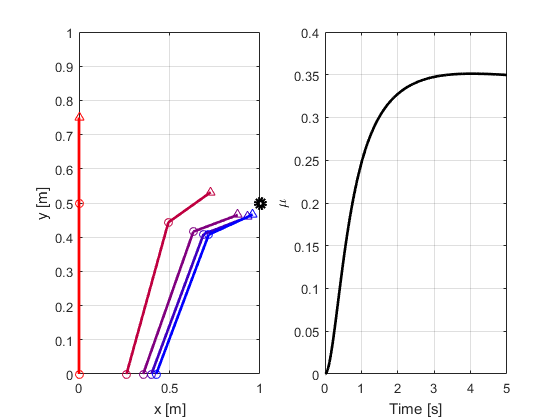
Simulating System
% Time and number of samples
Ts  = 0.01;
Tf  = 5.0;
t   = 0:Ts:Tf;
N   = numel(t);

% Joint state, manipulability index and points of interest
q   = zeros(3,N);
mu  = zeros(1,N);
p_a = zeros(2,N);
p_b = zeros(2,N);
p_c = zeros(2,N);

% Initial condition: vertical position
q(:,1) = [0.0; pi/2; 0];

% Arms length
L      = [0.5; 0.25];

% Gain and desired position
K      = [0.4; 1.0; 5.0];
p_d    = [1;0.5];

% Simulate kinematics control
figure(1);
subplot(1,2,1)
plot(p_d(1),p_d(2), 'ok', 'LineWidth',4), hold on;
for k=1:N

    % Compute the location of the points of interest
    [p_a(:,k), p_b(:,k), p_c(:,k)] = PRRKine(q(:,k), L);

    % Compute control action
    [q_dot_c, J] = PRRCtrl(q(:,k), L, p_d, K);

    % Evaluate the manipulability index
    mu(k) = det(J*J');

    % Plot trajectory: red to blue over time
    if k==1 || mod(k,floor(N/4))==0
        Color = [1;0;0]*(N-k)/N + [0;0;1]*(k/N);
        % Plot the three points
        plot(p_a(1,k),p_a(2,k),'o','Color',Color), hold on;
        plot(p_b(1,k),p_b(2,k),'o','Color',Color)
        plot(p_c(1,k),p_c(2,k),'^','Color',Color)

        % Plot the two links
        plot([p_a(1,k),p_b(1,k)],...
            [p_a(2,k),p_b(2,k)],'-', 'LineWidth',2,'Color',Color);
        plot([p_b(1,k),p_c(1,k)],...
            [p_b(2,k),p_c(2,k)],'-', 'LineWidth',2,'Color',Color);
    end

    % Integrate with forward Euler
    q(:,k+1) = q(:,k) + Ts*q_dot_c;
end
grid on, hold off;
xlim([0,1]); ylim([0,1])
xlabel('x [m]'), ylabel('y [m]');

% Plot manipulability index over time
subplot(1,2,2)
plot(t, mu, 'k', 'LineWidth',2);
grid on; hold off;
xlim([0,Tf]),
xlabel('Time [s]'), ylabel('\mu')
Get in Touch